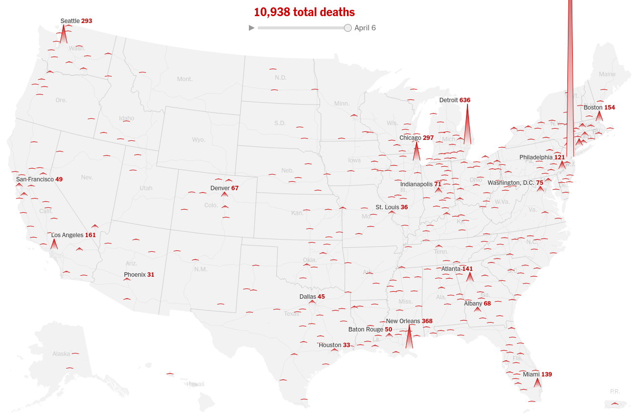
Latest epicenters of infection and death toll in the US
Geospatial map with custom SVG path as spikes showing the trends in cases in the last week and the death toll
Today we will make a very special graph that looks like the article See How the Coronavirus Death Toll Grew Across the U.S.

This will require us to use some special techniques using SVG Path elements.
import geopandas as gpd
import altair as alt
import pandas as pd
alt.renderers.set_embed_options(actions=True)
# NYT dataset
county_url = 'https://raw.githubusercontent.com/nytimes/covid-19-data/master/us-counties.csv'
cdf = pd.read_csv(county_url)
cdf.head()
# Shapefiles from us census
state_shpfile = './shapes/cb_2019_us_state_20m'
county_shpfile = './shapes/cb_2019_us_county_20m'
states = gpd.read_file(state_shpfile)
county = gpd.read_file(county_shpfile)
# Adding longitude and latitude in state data
states['lon'] = states['geometry'].centroid.x
states['lat'] = states['geometry'].centroid.y
# Adding longitude and latitude in county data
county['lon'] = county['geometry'].centroid.x
county['lat'] = county['geometry'].centroid.y
NYT publishes the data for New York City in a different way. So we will add custom FIPS for New York City and Puerto Rico too whose county level information is not present.
cdf.loc[cdf['county'] == 'New York City','fips'] = 1
cdf[cdf['county'] == 'New York City'].head()
cdf.loc[cdf['state'] == 'Puerto Rico', 'fips'] = 2
cdf[cdf['state'] == 'Puerto Rico'].head()
Extracting the latest cases and deaths -
aggregate = cdf.groupby('fips', as_index=False).agg({'county': 'first', 'date': 'last', 'state': 'last', 'cases': 'last', 'deaths': 'last'})
aggregate.head()
Combining the 5 boroughs - New York, Kings, Queens, Bronx and Richmond - into one and adding that spatial area in the geodatatrame
#New York City fips = 36005', '36047', '36061', '36081', '36085 which corresponds to New York, Kings, Queens, Bronx and Richmond
spatial_nyc = county[county['GEOID'].isin(['36005', '36047', '36061', '36081', '36085'])]
combined_nyc = spatial_nyc.dissolve(by='STATEFP')
alt.Chart(spatial_nyc).mark_geoshape(stroke='white', strokeWidth=3).encode() | alt.Chart(combined_nyc).mark_geoshape(stroke='white', strokeWidth=3).encode()
agg_nyc_data = spatial_nyc.dissolve(by='STATEFP').reset_index()
agg_nyc_data['GEOID'] = '1'
agg_nyc_data['fips'] = 1
agg_nyc_data['lon'] = agg_nyc_data['geometry'].centroid.x
agg_nyc_data['lat'] = agg_nyc_data['geometry'].centroid.y
county = gpd.GeoDataFrame(pd.concat([county, agg_nyc_data], ignore_index=True))
county['fips'] = county['GEOID']
county['fips'] = county['fips'].astype('int')
county.head()
msa = pd.read_csv('core_msa_list.csv', sep=";")
msa_shp = gpd.read_file('shapes/cb_2019_us_cbsa_500k/cb_2019_us_cbsa_500k.shp')
#msa[msa['CBSA Title'].str.startswith('New York')]
msa.head()
msa_shp.head()
msa['FIPS State Code'] = msa['FIPS State Code'].astype(str)
msa['FIPS County Code'] = msa['FIPS County Code'].astype(str)
state_fips_max_length = msa['FIPS State Code'].map(len).max()
county_fips_max_length = msa['FIPS County Code'].map(len).max()
msa['FIPS State Code'] = msa['FIPS State Code'].apply(lambda x: '0'*(state_fips_max_length - len(x))+x)
msa['FIPS County Code'] = msa['FIPS County Code'].apply(lambda x: '0'*(county_fips_max_length - len(x))+x)
msa['fips'] = msa['FIPS State Code']+msa['FIPS County Code']
msa['fips'] = msa['fips'].astype(float)
Now we will add a row for New York
nyc_temp = pd.DataFrame({'CBSA Code': 35620,'Metropolitan Division Code': None, 'CSA Code': 408, 'CBSA Title': None,'Metropolitan/Micropolitan Statistical Area': None, 'Metropolitan Division Title': None,'CSA Title': None,'County/County Equivalent': None, 'State Name': 'New York', 'FIPS State Code': 36, 'FIPS County Code': None, 'Central/Outlying County': None, 'fips': 1},index=[0])
msa = pd.concat([msa, nyc_temp], ignore_index=True)
msa
msa['CBSA Code'] = msa['CBSA Code'].astype(float)
msa[msa['fips'].isin(aggregate['fips']) == False]
# Puerto Rico does not provide data at county level. So we will have to do a similar exercise like NYC for PR and aggregate it statewise.
# But since in albersUsa projection PR is filtered anyways, we won't be doing that exercise right away. Once I figure out how to use custom projection in the default
# albersUsa projection that is used by Vega-Lite under the hood, we will include Puerto Rico
aggregate[aggregate['state'].str.startswith('Puerto')]
aggregate[aggregate['fips'].isin(msa['fips']) == False]
Now we will merge the aggregated data with msa since msa is expanded on fips(CBSA repeats), which is the only unique column.
msa = msa.merge(aggregate, how='inner', on='fips')
msa
msa.rename(columns={'CBSA Code': 'CBSAFP'}, inplace=True)
msa_shp['CBSAFP'] = msa_shp['CBSAFP'].astype(float)
msa_shp['lon'] = msa_shp['geometry'].centroid.x
msa_shp['lat'] = msa_shp['geometry'].centroid.y
Now we will aggregate the msa data on CBSAFP so that it becomes similar to msa_shp geodataframe
msa_agg = msa.groupby('CBSAFP', as_index=False).agg({'CBSA Title': 'first', 'State Name': 'last', 'date': 'last', 'cases': 'sum', 'deaths': 'sum'})
msa_agg.head()
Now we will merge msa_agg with msa and make the heights column that contains a custom SVG Path string per row, since right now Vega-Lite does not support "scaleY" as an encoding. In Vega, we don't have to do it this way, we can just provide a single svg path for an equilateral triangle and then stretch it(using scaleY) based on "cases" or "deaths".
msa_shp = msa_shp.merge(msa_agg, how='inner', on='CBSAFP')
msa_shp['height'] = msa_shp['deaths'].apply(lambda x: f"M -1.5 0 L0 -{x/50} L1.5 0" if pd.notnull(x) else "M -1.5 0 L0 0 L1.5 0")
msa_shp.head()
msa_shp.drop(['CSAFP', 'AFFGEOID', 'GEOID', 'LSAD', 'ALAND', 'AWATER'], axis=1, inplace=True)
msa_shp.head()
Let's finally plot this graph of deaths till now -
spikes = alt.Chart(msa_shp).transform_filter(alt.datum.deaths>0).mark_point(
fillOpacity=1,
fill=alt.Gradient(
gradient="linear",
stops=[alt.GradientStop(color='white', offset=0), alt.GradientStop(color='red', offset=0.5)],
x1=1,
x2=1,
y1=1,
y2=0
),
#dx=10,
#dy=-30,
strokeOpacity=1,
strokeWidth=1,
stroke='red'
).encode(
latitude="lat:Q",
longitude="lon:Q",
shape=alt.Shape("height:N", scale=None),
#tooltip=['CBSA Title:N', 'deaths:Q'],
#color = alt.condition(selection, alt.value('black'), alt.value('red'))
).project(
type='albersUsa'
).properties(
width=1200,
height=800
)
state = alt.Chart(states).mark_geoshape(fill='#ededed', stroke='white').encode(
).project(
type='albersUsa'
)
(state+spikes).configure_view(strokeWidth=0)